Excel Notes

Excellent LinkedIn Excel Tutorial

Excel Formulas and Functions Quick Tips


Piviot Table & Chart

Xlookup notes

Search for text

VBA Extract URL's from List

=ISEVEN(ROW())

Transpose Data Rows to Columns

How to Fill Down without dragging or incrementing

Here are the steps to fill down an entire column with a value without incrementing a number using a keyboard shortcut:

  1. Select the cell containing the value you want to copy.

  2. Press "Ctrl + C" to copy the value to the clipboard.

  3. Select the range of cells in the column where you want to paste the value, starting from the cell immediately below the cell with the copied value.

    you can also press Ctrl+ Shift+ Arrow down to select the entire column

  4. Press "Ctrl + Alt + V" to open the Paste Special dialog box.

  5. In the Paste Special dialog box, select "Values" under "Paste", and then select "Formats" under "Paste Special".

  6. Click on the "OK" button to apply the formatting to the selected cells.

This will paste the copied value into the selected range of cells without incrementing any numbers.

https://allthings.how/how-to-autofill-in-excel-without-dragging/


Search for NON ASCII Characters in Excel

=(SUMPRODUCT(--(UNICODE(MID(A2,ROW(INDIRECT("1:"&LEN(A2))),1))>=132))>0)


https://techcommunity.microsoft.com/t5/excel/how-to-filter-special-characters-in-excel/m-p/744698/highlight/true#M34246


=IF(SUMPRODUCT(--(CODE(MID(E2,ROW(INDIRECT("1:"&LEN(E2))),1))>127))>0,"Non-ASCII characters found","OK")


=ISNUMBER(SEARCH("apple",A1))

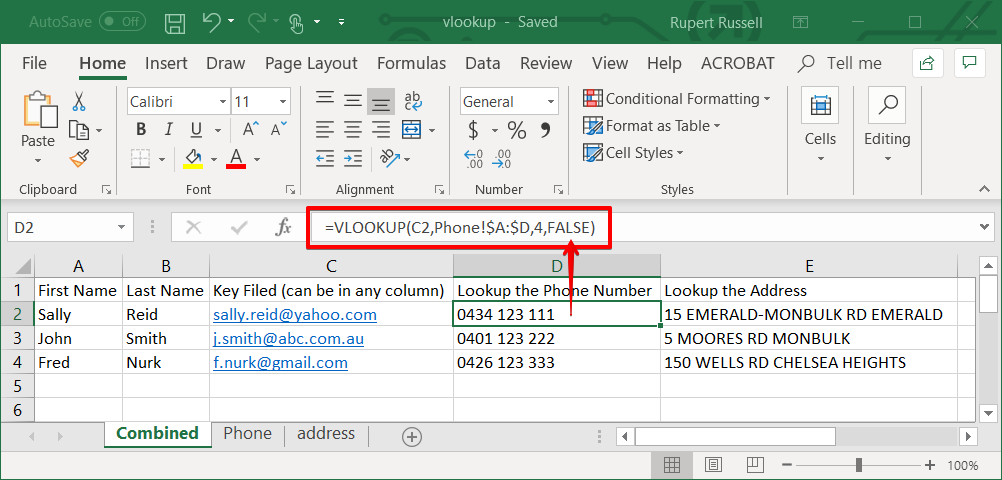
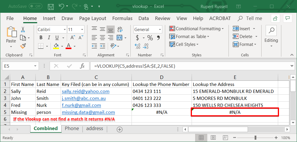
Vlookup is extremely useful when you want to combine data from multiple spreadsheets.

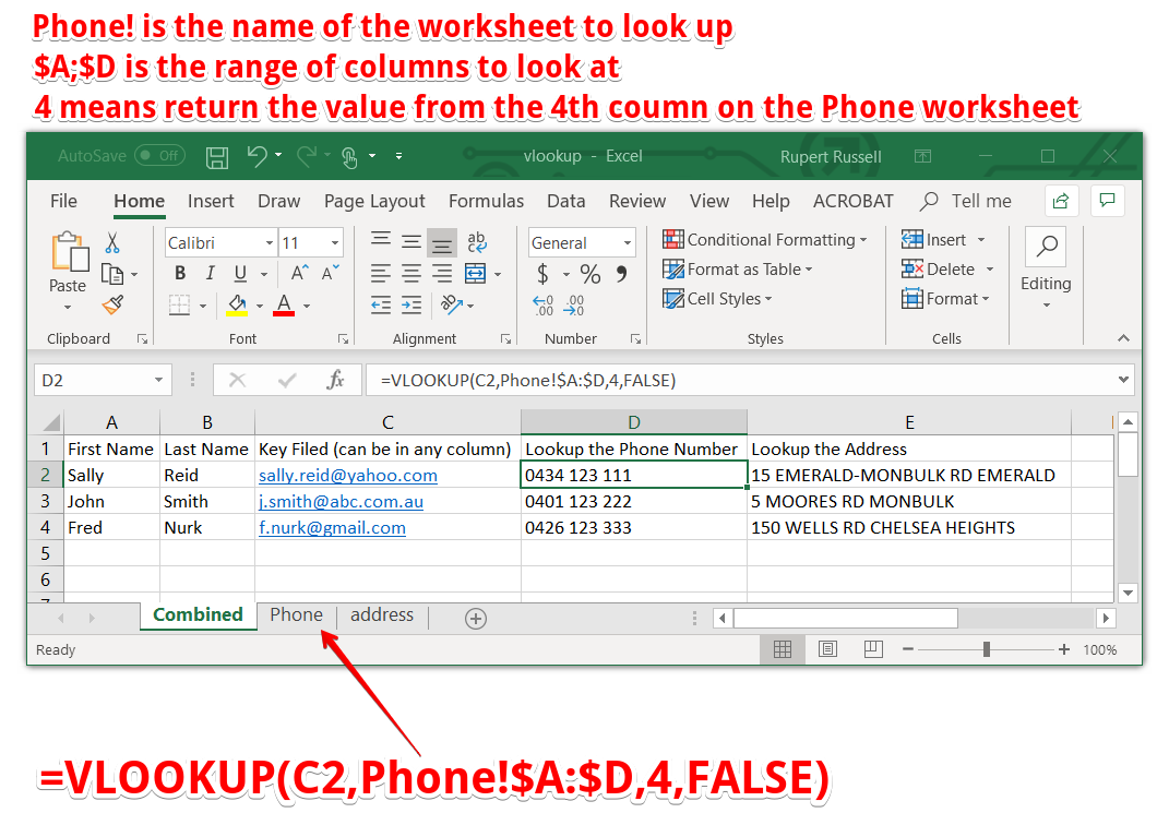
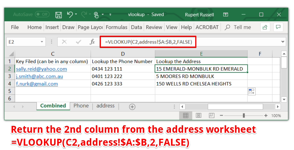
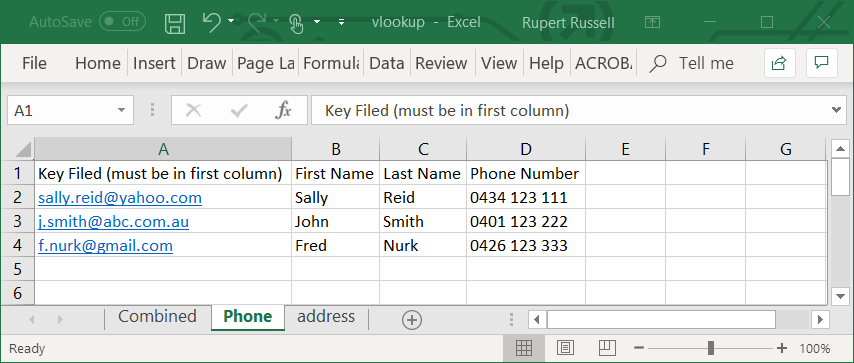
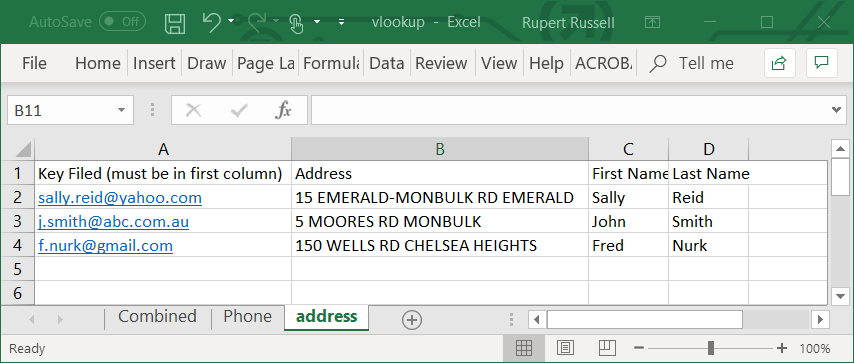
In the vlokup.xls file below I use VLOOKUP to look up the phone numbers, and addresses and combine them into a single workbook.

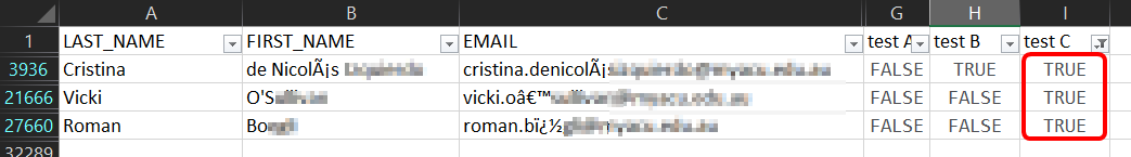
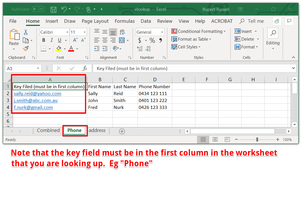
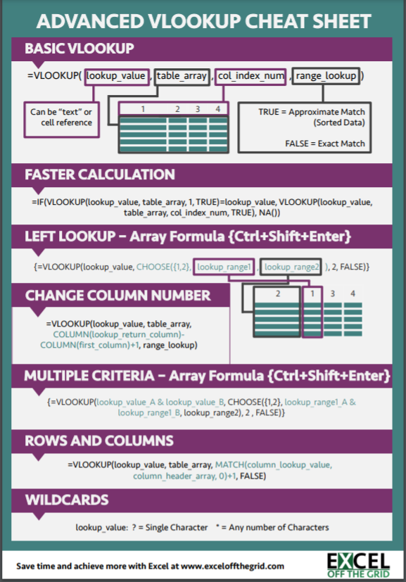
Things to note, the key field has to be in the first column in the worksheet that contains the lookup value

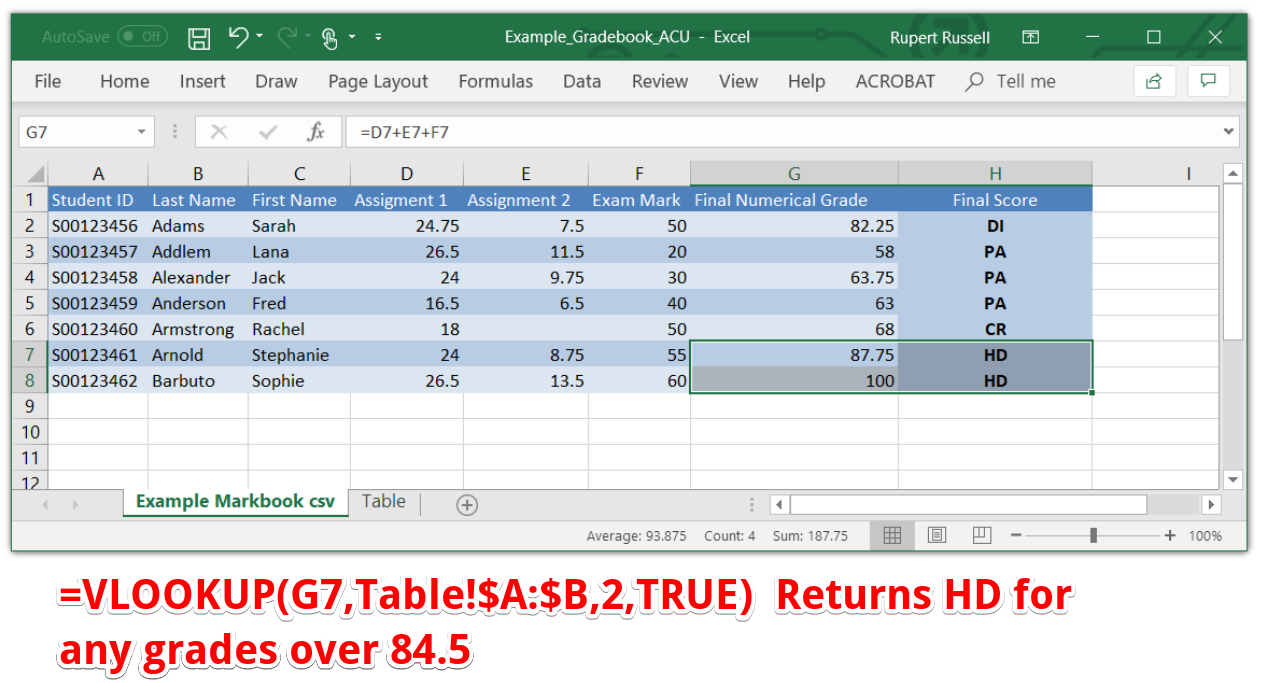
the word false in the formula =VLOOKUP(C2,Phone!$A:$D,4,FALSE) means return an exact match it is possible to rerun a match from a range of values see below for the Markbook example


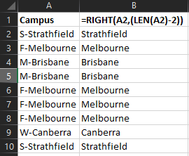
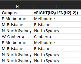
=RIGHT(A2,(LEN(A2)-2))
strip the first 2 characters from a string


how do you delete every 2nd row in an excel spreadsheet https://trumpexcel.com/delete-every-other-row-excel/


See my Markbook Notes for an example of using Vlookup to return a single value that matches a range

EG Grades


248K subscribers
SUBSCRIBE
The ultimate compilation of Excel tips and tricks to enhance your productivity using Excel. Updated for 2020! I've combined long-established tips and tricks with new ones Microsoft added in 2019 and 2020. You'll find solutions to the most common challenges you face in Excel. Support me with your Amazon purchases, click here: https://amzn.to/2Kxp533 Contents 0:00 1. Move Data 0:35 2. XLOOKUP() 1:04 3. Filter List 2:24 4. Ideas 3:04 5. Remove Blanks 3:54 6. Quick Analysis Tool 4:28 7. AutoFit Column Width 5:27 8. Absolute Cell Reference 5:57 9. Paste Special Values 7:19 10. Drop-Down List 8:05 11. FILTER() 9:15 12. Remove Duplicates 10:43 13. Difference Between Lists 11:31 14. Flash Fill 12:15 15. AutoFill 13:06 16. Data Types 13:53 17. Transpose 15:11 18. Freeze Panes 15:37 19. Text to Columns 16:27 20. Recommended Pivot table 17:25 21. Slicers 18:04 22. Conditional Formatting 19:01 23. IF() 20:29 24. 3D References 21:12 25. Forecast Sheet 22:45 26. SUMIFS() 24:00 27. IFERROR() 25:15 28. Ctrl-Arrow Keys 26:03 29. Filled Maps 26:26 30. PMT() 27:13 31. Show Formulas 28:20 32. Advanced Select 29:10 33. Named Range Shortcut 29:56 34. Hide Cells 30:47 35. COUNTBLANK() 31:30 36. Natural Language Query 31:59 37. Goal Seek 33:08 38. Insert Screenshot 34:30 39. Power Pivot 35:14 40. 3D Maps 36:16 41. ISBLANK() 39:08 42. Analysis ToolPak 39:45 43. CONVERT() 40:48 44. Get Data from Web 41:24 45. People Graph 42:59 46. SORT() 44:18 47. Status Bar Info 45:36 48. Insert Multiple Rows 46:22 49. CHOOSE() 46:53 50. UNIQUE() 48:50

Note: you can also use Vlookup to merge data from 2 worksheets in Excel

Combine data using vlookup 11 KB Ziped with Winzip

https://echo360.org.au/media/ac5acbc4-ca1a-4139-bf47-ecc67a508814/public


Advanced Vlookup options from

https://exceloffthegrid.com/vlookup-what-does-the-true-false-statement-do/


How to use regular expressions in Excel

by  | Jun 15, 2021 | Excel Tips & Tricks

How-to-use-regular-expressions-in-Excel (zip file with macros)


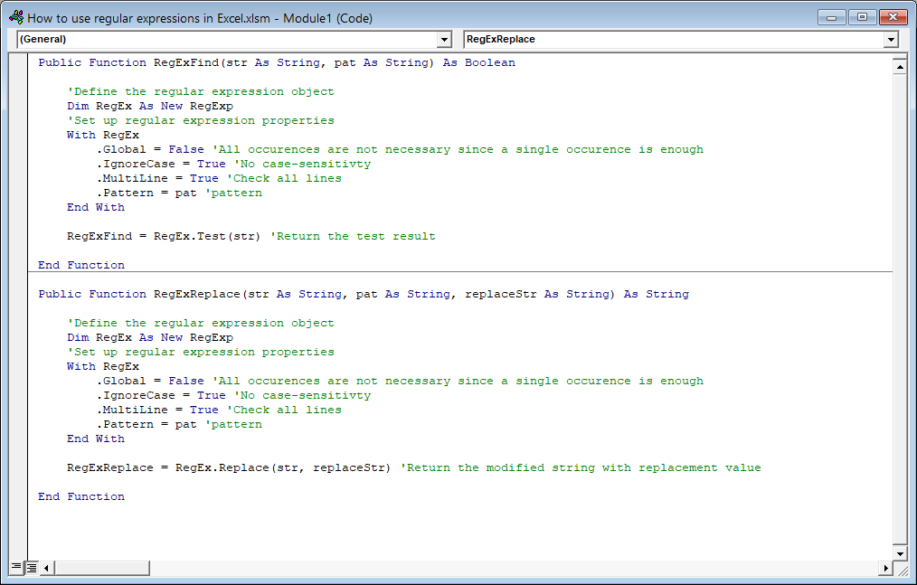
Public Function RegExFind(str As String, pat As String) As Boolean

'Define the regular expression object
Dim RegEx As New RegExp
'Set up regular expression properties
With RegEx
.Global = False 'All occurences are not necessary since a single occurence is enough
.IgnoreCase = True 'No case-sensitivty
.MultiLine = True 'Check all lines
.Pattern = pat 'pattern
End With

RegExFind = RegEx.Test(str) 'Return the test result

End Function


Public Function RegExReplace(str As String, pat As String, replaceStr As String) As String

'Define the regular expression object
Dim RegEx As New RegExp
'Set up regular expression properties
With RegEx
.Global = False 'All occurences are not necessary since a single occurence is enough
.IgnoreCase = True 'No case-sensitivty
.MultiLine = True 'Check all lines
.Pattern = pat 'pattern
End With

RegExReplace = RegEx.Replace(str, replaceStr) 'Return the modified string with replacement value

End Function

Excel – measure distance between any points on Earth

Alt and type 0176 on Windows with a numeric keypad. ° Degree Symbol

=6371 * ACOS(SIN([latitude of 1st location]*PI()/180)*SIN([latitude of 2nd location]*PI()/180) + COS([latitude of 1st location]*PI()/180) * COS([latitude of 2nd location]*PI()/180)*COS([longitude of 2nd location]* PI()/180-[longitude of 1st location] *PI()/180))

The formula is relatively long, but once executed, you get precise distance in kilometers. I will not go into explaining the details of the formula, but one thing I will call out: Note that the first number 6371 is Earth’s radius in kilometers. If you prefer to calculate in miles, then substitude the radius to 3959 miles.
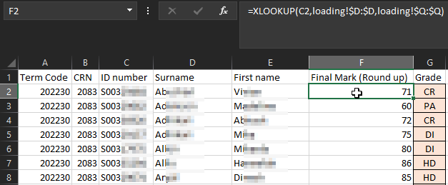


XLOOKUP Notes


We want to populate the Final Mark (Round up) column using data from another worksheet

The Xlookup formula is the best way to do this. it lets us take a value from one worksheet and look up (find) the matchig value in any column
in another worksheet and then return a vlaue from the same row in another column.

In this example we are reading the ID number from cell C2 and then finding that ID number is column D in a 2nd worksheet called Loading and
returning the Final Mark (Round up) from Column Q.

=XLOOKUP(C2,loading!$D:$D,loading!$Q:$Q)


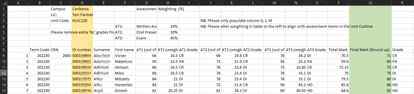
The loading tab contains the following data: we are only interested in Column D which contains the student numbers and column Q withic contains the Final Mark (Round up).


Return from Column A or B not A+B

=IF((AND(A2>0,B2>0)),"DANGER",A2+B2)